Excel アドインで遅延注文にフラグを設定したり、負の値を強調表示したり、セル値を変更せずに傾向を視覚化したりする必要がある場合は、条件付き書式を使用します。 この記事では、一般的なルールの種類の作成、既存のルールの更新、ルールの優先順位の制御、ルールのクリアを行う方法について説明します。 Excel の組み込みの条件付き書式エクスペリエンスの背景については、「 条件付き書式を使用して Excel の情報を強調表示する 」および「 数式を使用して Excel で条件付き書式を適用する」を参照してください。
ヒント
関連するタスクについては、「 Excel JavaScript API を使用して範囲形式を設定する」および「Excel範囲にデータ検証を追加する」を参照してください。
重要な点
-
Range.conditionalFormatsを使用して、範囲の条件付き書式ルールを作成および管理します。 - 各
ConditionalFormatオブジェクトでは、cellValue、colorScale、iconSetなど、1 つの規則の種類のみを使用できます。 -
priorityとstopIfTrueを使用して、複数のルールが同じ範囲でどのように相互作用するかを制御します。 -
clearFormatまたはclearAllを使用して、書式設定の詳細またはルール全体を削除します。
条件付き書式のプログラムによる制御
Range.conditionalFormats プロパティは、範囲に適用される ConditionalFormat オブジェクトのコレクションです。
ConditionalFormat オブジェクトには、ConditionalFormatType に基づいて適用する形式を定義するプロパティが含まれています。
cellValuecolorScalecustomdataBariconSetpresettextComparisontopBottom
これらの書式設定プロパティにはそれぞれ、対応する *OrNullObject バリアントが存在します。 そのパターンの詳細については、「 *OrNullObject メソッド」を参照してください。
ConditionalFormat オブジェクトに設定できる書式の種類は 1 つだけです。
type プロパティ (ConditionalFormatType 列挙値) によって、書式の種類が決まります。 条件付き書式を範囲に追加するときに type を設定します。
一般的な条件付き書式ルールを作成する
conditionalFormats.addを使用して、条件付き書式を範囲に追加します。 条件付き書式を追加したら、その形式に固有のプロパティを設定します。 次のシナリオは、ワークシートに適応できる一般的なルールの種類を示しています。
セルの値
セルの値の条件付き書式では、ConditionalCellValueRule 内の 1 つまたは 2 つの数式の結果に基づいて、ユーザー定義の書式を適用することができます。
operator プロパティは、結果の式が書式設定にどのように関連するかを定義する ConditionalCellValueOperator です。
次に、範囲内の 0 未満の値すべてに赤のフォント色を適用する例を示します。

await Excel.run(async (context) => {
    const sheet = context.workbook.worksheets.getItem("Sample");
    const range = sheet.getRange("B21:E23");
    const conditionalFormat = range.conditionalFormats.add(
        Excel.ConditionalFormatType.cellValue
    );

    // Set the font of negative numbers to red.
    conditionalFormat.cellValue.format.font.color = "red";
    conditionalFormat.cellValue.rule = { formula1: "=0", operator: "LessThan" };

    await context.sync();
});
カラー スケール
カラー スケールの条件付き書式では、データの範囲に色のグラデーションを適用することができます。
ColorScaleConditionalFormat 上の criteria プロパティは、3 つの ConditionalColorScaleCriterion を定義します: minimum、maximum、midpoint (オプション) です。 各基準スケール ポイントには、次の 3 つのプロパティがあります。
-
color- エンドポイントに対する HTML カラー コード。 -
formula- エンドポイントを表す数値または数式。 この値は、typeがlowestValueまたはhighestValueの場合にnullされます。 -
type- 数式の評価方法。highestValueとlowestValueは、書式設定対象の範囲内の値を参照します。
次に、範囲内の色を青から黄色、そして赤に設定する例を示します。
minimum と maximum はそれぞれ最低値と最高値を表すものであり、null 数式を使用します。
midpoint では、 percentage 型と "=50" の数式が使用されるため、最も黄色のセルが平均値になります。

await Excel.run(async (context) => {
    const sheet = context.workbook.worksheets.getItem("Sample");
    const range = sheet.getRange("B2:M5");
    const conditionalFormat = range.conditionalFormats.add(
          Excel.ConditionalFormatType.colorScale
    );

    // Color the backgrounds of the cells from blue to yellow to red based on value.
    const criteria = {
          minimum: {
               formula: null,
               type: Excel.ConditionalFormatColorCriterionType.lowestValue,
               color: "blue"
          },
          midpoint: {
               formula: "50",
               type: Excel.ConditionalFormatColorCriterionType.percent,
               color: "yellow"
          },
          maximum: {
               formula: null,
               type: Excel.ConditionalFormatColorCriterionType.highestValue,
               color: "red"
          }
    };
    conditionalFormat.colorScale.criteria = criteria;

    await context.sync();
});
Custom
ユーザー設定の条件付き書式では、任意の複雑な数式に基づいて、ユーザー定義の書式をセルに適用することができます。 ConditionalFormatRule オブジェクトでは、さまざまな表記で数式を定義することができます。
-
formula- 標準の表記法。 -
formulaLocal- ユーザーの言語に基づいてローカライズされます。 -
formulaR1C1- R1C1 スタイルの表記法。
次の例では、セルよりも大きい値を持つセルのフォントを緑色に色付けします。

await Excel.run(async (context) => {
    const sheet = context.workbook.worksheets.getItem("Sample");
    const range = sheet.getRange("B8:E13");
    const conditionalFormat = range.conditionalFormats.add(
         Excel.ConditionalFormatType.custom
    );

    // If a cell has a higher value than the one to its left, set that cell's font to green.
    conditionalFormat.custom.rule.formula = '=IF(B8>INDIRECT("RC[-1]",0),TRUE)';
    conditionalFormat.custom.format.font.color = "green";

    await context.sync();
});
データ バー
データ バーの条件付き書式では、セルにデータ バーを追加することができます。 既定では、範囲内の最小値と最大値は、データ バーの境界と比例サイズを形成します。
DataBarConditionalFormat オブジェクトには、バーの外観を制御するいくつかのプロパティがあります。
次に、範囲内でデータ バーを左から右にグラデーション表示する例を示します。

await Excel.run(async (context) => {
    const sheet = context.workbook.worksheets.getItem("Sample");
    const range = sheet.getRange("B8:E13");
    const conditionalFormat = range.conditionalFormats.add(
         Excel.ConditionalFormatType.dataBar
    );

    // Give left-to-right, default-appearance data bars to all the cells.
    conditionalFormat.dataBar.barDirection = Excel.ConditionalDataBarDirection.leftToRight;
    await context.sync();
});
アイコン セット
アイコン セットの条件付き書式では、Excel のアイコンを使用してセルを強調表示することができます。
criteria プロパティは、挿入するシンボルと挿入条件を定義する ConditionalIconCriterion の配列です。 この配列は、既定のプロパティを持つ条件要素で自動的に事前設定されます。 個々のプロパティを上書きすることはできません。 代わりに、criteria オブジェクト全体を置き換えます。
次に、3 つの三角形のアイコン セットを範囲に適用する例を示します。

await Excel.run(async (context) => {
    const sheet = context.workbook.worksheets.getItem("Sample");
    const range = sheet.getRange("B8:E13");
    const conditionalFormat = range.conditionalFormats.add(
         Excel.ConditionalFormatType.iconSet
    );

    const iconSetCF = conditionalFormat.iconSet;
    iconSetCF.style = Excel.IconSet.threeTriangles;

    /*
       With a "three*" icon set style, such as "threeTriangles", the third
        element in the criteria array (criteria[2]) defines the "top" icon;
        e.g., a green triangle. The second (criteria[1]) defines the "middle"
        icon, The first (criteria[0]) defines the "low" icon, but it can often
        be left empty as this method does below, because every cell that
       does not match the other two criteria always gets the low icon.
    */
    iconSetCF.criteria = [
        {},
          {
            type: Excel.ConditionalFormatIconRuleType.number,
            operator: Excel.ConditionalIconCriterionOperator.greaterThanOrEqual,
            formula: "=700"
          },
          {
            type: Excel.ConditionalFormatIconRuleType.number,
            operator: Excel.ConditionalIconCriterionOperator.greaterThanOrEqual,
            formula: "=1000"
          }
    ];

    await context.sync();
});
事前設定の条件
事前設定の条件付き書式では、選択した標準ルールに基づいて、ユーザー定義の書式を範囲に適用することができます。 ConditionalPresetCriteriaRule の ConditionalFormatPresetCriterion は、これらの規則を定義します。
次の例では、セルの値が範囲の平均より少なくとも 1 つの標準偏差である場合は、フォントを白に色付けします。

await Excel.run(async (context) => {
    const sheet = context.workbook.worksheets.getItem("Sample");
    const range = sheet.getRange("B2:M5");
    const conditionalFormat = range.conditionalFormats.add(
         Excel.ConditionalFormatType.presetCriteria
    );

    // Color every cell's font white that is one standard deviation above average relative to the range.
    conditionalFormat.preset.format.font.color = "white";
    conditionalFormat.preset.rule = {
         criterion: Excel.ConditionalFormatPresetCriterion.oneStdDevAboveAverage
    };

    await context.sync();
});
テキストの比較
テキストの比較の条件付き書式では、条件として文字列比較を使用します。
rule プロパティは、セルと比較する文字列を定義する ConditionalTextComparisonRule と、比較の種類を指定する演算子です。
次の例では、セルのテキストに "Delayed" が含まれている場合に、フォントの色を赤で書式設定します。

await Excel.run(async (context) => {
    const sheet = context.workbook.worksheets.getItem("Sample");
    const range = sheet.getRange("B16:D18");
    const conditionalFormat = range.conditionalFormats.add(
         Excel.ConditionalFormatType.containsText
    );

    // Color the font of every cell containing "Delayed".
    conditionalFormat.textComparison.format.font.color = "red";
    conditionalFormat.textComparison.rule = {
         operator: Excel.ConditionalTextOperator.contains,
         text: "Delayed"
    };

    await context.sync();
});
上位/下位
上位/下位の条件付き書式では、範囲内の上位または下位の値を持つセルに書式を適用することができます。
ConditionalTopBottomRule の種類である rule プロパティでは、条件を上位または下位のどちらで設定するのか、また順位とパーセンテージのどちらでランクを決定するのかを、設定します。
次に、範囲内で一番上位の値を持つセルの色を緑に設定する例を示します。
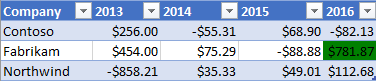
await Excel.run(async (context) => {
    const sheet = context.workbook.worksheets.getItem("Sample");
    const range = sheet.getRange("B21:E23");
    const conditionalFormat = range.conditionalFormats.add(
         Excel.ConditionalFormatType.topBottom
    );

    // For the highest valued cell in the range, make the background green.
    conditionalFormat.topBottom.format.fill.color = "green"
    conditionalFormat.topBottom.rule = { rank: 1, type: "TopItems"}

    await context.sync();
});
条件付き書式ルールを変更する
ConditionalFormat オブジェクトには、コードが設定した後で条件付き書式ルールを変更する複数のメソッドが用意されています。
- changeRuleToCellValue
- changeRuleToColorScale
- changeRuleToContainsText
- changeRuleToCustom
- changeRuleToDataBar
- changeRuleToIconSet
- changeRuleToPresetCriteria
- changeRuleToTopBottom
次の例は、前の一覧の changeRuleToPresetCriteria メソッドを使用して、既存の条件付き書式ルールを事前設定された条件ルールの種類に変更する方法を示しています。 指定された範囲には、条件付き書式ルールが既に存在している必要があります。 範囲にルールがない場合、変更メソッドは新しいルールを適用しません。
await Excel.run(async (context) => {
    const sheet = context.workbook.worksheets.getItem("Sample");
    const range = sheet.getRange("B2:M5");

    // Retrieve the first existing `ConditionalFormat` rule on this range.
    // Note: The specified range must have an existing conditional format rule.
    const conditionalFormat = range.conditionalFormats.getItemOrNullObject("0");

    // Change the conditional format rule to preset criteria.
    conditionalFormat.changeRuleToPresetCriteria({
        criterion: Excel.ConditionalFormatPresetCriterion.oneStdDevAboveAverage,
    });
    conditionalFormat.preset.format.font.color = "red";

    await context.sync();
});
複数の書式と優先度
範囲には、複数の条件付き書式を適用することができます。 フォント色が異なるなど、書式間で競合する要素がある場合、ある 1 つの書式のみがその競合要素に対して適用されます。
ConditionalFormat.priority プロパティは、優先する形式を定義します。 Priority は、 ConditionalFormatCollection内のインデックスと等しい数値であり、形式を作成するときに設定します。
priority値が小さい場合は、優先度が高いことを意味します。
次に、選択されるフォント色が 2 つの書式間で競合している例を示します。 負の数値は太字のフォントを取得しますが、赤いフォントは取得しません。これは、優先順位が青色のフォントを与える形式になるためです。

await Excel.run(async (context) => {
    const sheet = context.workbook.worksheets.getItem("Sample");
    const temperatureDataRange = sheet.tables.getItem("TemperatureTable").getDataBodyRange();


    // Set low numbers to bold, dark red font and assign priority 1.
    const presetFormat = temperatureDataRange.conditionalFormats
        .add(Excel.ConditionalFormatType.presetCriteria);
    presetFormat.preset.format.font.color = "red";
    presetFormat.preset.format.font.bold = true;
    presetFormat.preset.rule = { criterion: Excel.ConditionalFormatPresetCriterion.oneStdDevBelowAverage };
    presetFormat.priority = 1;

    // Set negative numbers to blue font with green background and set priority 0.
    const cellValueFormat = temperatureDataRange.conditionalFormats
        .add(Excel.ConditionalFormatType.cellValue);
    cellValueFormat.cellValue.format.font.color = "blue";
    cellValueFormat.cellValue.format.fill.color = "lightgreen";
    cellValueFormat.cellValue.rule = { formula1: "=0", operator: "LessThan" };
    cellValueFormat.priority = 0;

    await context.sync();
});
同時使用不可の条件付き書式
ConditionalFormat の stopIfTrue を使用すると、優先度の低い条件付き書式を範囲に適用しないように設定することができます。 コードが stopIfTrue === true の条件付き書式を範囲に適用する場合、書式の詳細が矛盾しない場合でも、後続の条件付き書式は適用されません。
次に、2 つの条件付き書式が範囲に追加されている例を示します。 負の数値には、他の書式条件が true であるかどうかに関係なく、淡い緑色の背景を持つ青いフォントがあります。

await Excel.run(async (context) => {
    const sheet = context.workbook.worksheets.getItem("Sample");
    const temperatureDataRange = sheet.tables.getItem("TemperatureTable").getDataBodyRange();

    // Set low numbers to bold, dark red font and assign priority 1.
    const presetFormat = temperatureDataRange.conditionalFormats
        .add(Excel.ConditionalFormatType.presetCriteria);
    presetFormat.preset.format.font.color = "red";
    presetFormat.preset.format.font.bold = true;
    presetFormat.preset.rule = { criterion: Excel.ConditionalFormatPresetCriterion.oneStdDevBelowAverage };
    presetFormat.priority = 1;

    // Set negative numbers to blue font with green background and
    // set priority 0, but set stopIfTrue to true, so none of the
    // formatting of the conditional format with the higher priority
    // value will apply, not even the bolding of the font.
    const cellValueFormat = temperatureDataRange.conditionalFormats
        .add(Excel.ConditionalFormatType.cellValue);
    cellValueFormat.cellValue.format.font.color = "blue";
    cellValueFormat.cellValue.format.fill.color = "lightgreen";
    cellValueFormat.cellValue.rule = { formula1: "=0", operator: "LessThan" };
    cellValueFormat.priority = 0;
    cellValueFormat.stopIfTrue = true;

    await context.sync();
});
条件付き書式ルールをクリアする
特定の条件付き書式ルールから書式プロパティを削除するには、ConditionalRangeFormat オブジェクトの clearFormat メソッドを使用します。
clearFormat メソッドは、書式設定なしで書式設定規則を作成します。
特定の範囲またはワークシート全体からすべての条件付き書式ルールを削除するには、ConditionalFormatCollection オブジェクトの clearAll メソッドを使用します。
次の例は、 clearAll メソッドを使用してワークシートからすべての条件付き書式を削除する方法を示しています。
await Excel.run(async (context) => {
    const sheet = context.workbook.worksheets.getItem("Sample");
    const range = sheet.getRange();
    range.conditionalFormats.clearAll();

    await context.sync();
});
関連項目
GitHub で Microsoft と共同作業する
このコンテンツのソースは GitHub にあります。そこで、issue や pull request を作成および確認することもできます。 詳細については、共同作成者ガイドを参照してください。
Office Add-ins